python for microbiology

by a medical lab scientist learning programming in grad school

When I first heard “Python for microbiology”, my immediate thought was, “how and why”? I’d spent the last half a decade in the clinical lab - now someone was suggesting that I could automate parts of my job with a few lines of code. Skepticism aside, I dove in. And honestly? It changed the way I see the lab.

It started with something small; programming a CBC counter, then counting colony-forming units from an agar plate. Normally, I’d manually record these results while charting for patients. Its tedious and repetitive.

I opened python, typed out a few commands and ran a loop that read an excel file of plate counts I created. Ten minutes later, the output was neatly summarized , averages calculated, and a simple graph plotted.

Today, I want to walk you through a practical mini project I created. This simple python project takes organism and antibiotic resistance profiles, organizes them, and helps visualize patterns.

---

Getting Started: Your First Data Set

Before we can automate anything, we need data.. For this project, I created a mini dataset of bacterial culture results. Each row represents a single patient sample and includes:

• organism

• sample source

• growth results (CFU/mL)

• antibiotic resistance profile

Here’s an example I created in Python using pandas.

#step 1 - Create a dataframe of urine culture reads
import pandas as pd

import pandas as pd

culture = {
    “Specimen_ID”: [”UC001”, “UC002”, “UC003”, “UC004”, “UC005”, “UC006”, “UC007”, “UC008”, “UC009”, “C010”], 
    “Specimen_Type”: [”Urine”] * 10, 
    “Organism”:[
        “Escherichia coli”,
        “No growth”,
        “Klebsiella pneumonia”,
        “Mixed flora”,
        “Escherichia coli”,
        “Enterococcus faecalis”,
        “No growth”,
        “Escherichia coli”,
        “Pseudomonas aeruginosa”,
        “Mixed flora”
    ],
    “Colony_Couny_CFU_mL” : [100000, 0, 800000, 20000, 1500000, 70000, 0, 120000, 60000, 30000],
    “Antibiotic_Resistance_Profile”:[
        “Sensitive to all”, “-”,
        “Resistant to ampicillin”, “-”,
        “Resistant to TMP-SMX”, 
        “Sensitive to all”, “-”,
        “Resistant to ciprofloxacin”, “-” 
        “Resistant to multiple”, “-”
    ]
}

df = pd.DataFrame(culture)
print(df.head)At this point, you have a small, manageable dataset to experiment with. 

---

Step 1: Cleaning your Data

One of the first lessons in data analysis is: garbage in, garbage out.

Before running analysis, we need to clean our data. (in this case, remove any fields that are blank):

#Ensure no missing values
df["Antibiotic_Resistance_Profile"] = df["Antibiotic_Resistance_Profile"].fillna("").astype(str)

This prevents errors later when pulling antibiotic profiles.

---

Step 2 : Summarizing Results & Antibiotic Resistance Profiles

Now comes the fun part. Let’s extract which antibiotics each organism is resistant to and count occurrences.

#total number of specimens
total = len(df)

#count positive vs negative
positive = df[df[”Organism”] != “No growth”].shape[0]
negative = df[df[”Organism”] == “No growth”].shape[0]

print (f”Total specimens: {total}”)
print(f”Positive cultures: {positive}”)
print(f”Negative cultures: {negative}”)
print(f”Positivity rate: {(positive/total)*100:.1f}%”)


#Top Organisms
organism_counts = df[”Organism”].value_counts().reset_index()
organism_counts.columns = [”Organism”, “Count”]
print(organism_counts)

#Step 4 - Antibiotic Resistance Summary
import re
#extract all antibiotic names from text
antibiotics = []
for profile in df[”Antibiotic_Resistance_Profile”]:
    found = re.findall(r”Resistant to (\w+[-]?\w+)”, profile)
    antibiotics.extend (found)
res_df = pd.Series(antibiotics).value_counts().reset_index()
res_df_columns = [”Antibiotic”, “Resistance_Count”]

print(res_df)

What this does:

• Summarizes each organism and it’s growth pattern

• uses “re” to search each antibiotic profile for phrases like “Resistant to AMP”.

• Pulls out the antibiotic names

• counts how many times each antibiotic appears across samples.

In just a few lines, you now have a summary table for resistance trends.

#Output

Total specimens: 10
Positive cultures: 8
Negative cultures: 2
Positivity rate: 80.0%
                 Organism  Count
0        Escherichia coli      3
1               No growth      2
2             Mixed flora      2
3    Klebsiella pneumonia      1
4   Enterococcus faecalis      1
5  Pseudomonas aeruginosa      1
           index  count
0     ampicillin      1
1        TMP-SMX      1
2  ciprofloxacin      1
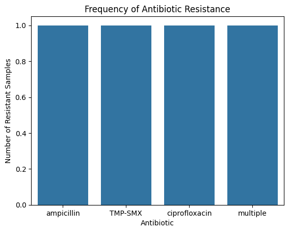
3       multiple      1

---

Step 3: Visualizing Resistance (Optional challenge)

As lab scientists, we know numbers tell a story, but visuals tell it faster.

import matplotlib.pyplot as plt
import seaborn as sns

sns.barplot(x=”index”, y=”count”, data=res_df)
plt.title(”Frequency of Antibiotic Resistance”)
plt.ylabel(”Number of Resistant Samples”)
plt.xlabel(”Antibiotic”)
plt.show()

Even a small dataset reveals patterns: maybe r(if our dataset was larger) AMP resistance is high in E.coli, or OXA resistance is prominent in S. aureus.

Imagine doing this on a hospital’s microbiology dataset for a week. Our findings would probably be a lot more realistic as we add in more and more data points.

Step 4 : Adding Complexity (Optional)

Once you’re comfortable, you can expand our project.

• Track resistance trends by organism

• Count resistance per organism

• incorporate growth results to see correlations between growth positivity and resistance patterns.

The goal isn’t to make you a software engineer (HAHA) .

It’s to make lab analyses more intuitive and insightful.

---

From working on this mini project, here’s some takeaways.

• Python makes repetitive tasks painless when we use functions.

• Your lab data has stories to tell. Resistance trends, outbreak patterns, and anomalies become visible when you automate analysis.

• Start small. Even a tiny dataset teaches core concepts of data cleaning and visualization.

• Lab experience + Coding = superpower. You already understand clinical context - python just amplifies your insight.

---

If you’re thinking about learning coding:

• Start with projects related to what you do everyday. Seeing results and understanding how code can solve problems you are already familiar with is motivating. Try to find one repetitive task and use python to automate it.

• Small steps matter. Write tiny scripts, run them, debug, repeat. Complexity can come later.

• Translate your lab knowledge to understand any potential errors. Python errors aren’t failures, they’re hints to guide you to correct logic (or syntax). A “QC/control failure” in the lab is like an exception in code. Both require review and interpretation.

• Visualize your data. Graphs and plots make trends obvious. They also make your work communicable to peers.

Learning python wasn’t instant! I struggled with syntax, loops and data frames for several months. My first script didn’t even run. My second crashed halfway through. I wanted to quit on so many occasions.

But here’s the thing: lab work had already trained me for this. I knew what persistence looked like. I knew what troubleshooting meant. I eventually learned to debug scripts like I troubleshoot instruments : methodically and step-by-step.

And slowly, the programming language became familiar. I started seeing patterns: for loops became routine, if statements were like decision trees, and functions felt like mini-procedures.

Python is not magic. Its a tool for understanding data. The same way we identify bacteria under a lens, Python helps us see patterns in lab data we couldn’t notice before. Even if you never use programming professionally, learning to automate small analyses - like bacterial culture summaries- can save time, reduce errors, and make you a more efficient lab scientist.

---

Try to recreate this mini project on new datasets.

Share your visualizations and insights - you might notice trends that haven’t been spotted yet!

Stay tuned for more mini projects

x Larae